Part 1: Fundamentals of data import, structuring, and plotting in tidyverse
by Vikram B. Baliga, Andrea Gaede and Shreeram Senthivasan
Last updated on 2019-11-29 09:54:06
Source:vignettes/group-01_Fundamentals-data-wrangling-tidyverse.Rmd
group-01_Fundamentals-data-wrangling-tidyverse.RmdIntroduction
This vignette is Part 1 of 3 for an R workshop created for BIOL 548L, a graduate-level course on data visualization taught at the University of British Columbia.
When the workshop runs, we split students into three groups with successively increasing levels of difficulty. We recommend everyone starts here and works through the code that follows. This vignette shows users how to load a clean data file into R and make boxplots and scatterplots. Once you are comfortable with the contents of this page, please feel free to move on to Part 2 and ultimately to Part 3 (which we recommend going through only after completing Part 2) here.
All code and contents of this vignette were written together by Vikram B. Baliga, Andrea Gaede and Shreeram Senthivasan.
Learning Objectives:
- Determine how to import and control data stored in different filetypes
- Understand the best practices for structuring data in tidyverse/ggplot
- Construct basic plots using ggplot
Load or install & load necessary packages
Before running the code below, make sure you have the necessary packages loaded. If you do not have the packages listed below installed on your computer, then download them from the CRAN site using install.packages() and then load them with library() as shown below.
library(ubcBIOL548L)
library(gapminder)
library(ggplot2)
library(tidyr)
library(dplyr)
#>
#> Attaching package: 'dplyr'
#> The following objects are masked from 'package:stats':
#>
#>     filter, lag
#> The following objects are masked from 'package:base':
#>
#>     intersect, setdiff, setequal, union
library(tibble)
library(readr)
library(readxl)
Data sets
You can get all data used in this vignette (and the other two!) by downloading this zip file.
Importing and peeking at data:
Import data using base R command, and give it the name my_data
Take a look at your data
# Structure
str(my_data)
#> 'data.frame':    1704 obs. of  6 variables:
#>  $ country  : Factor w/ 142 levels "Afghanistan",..: 1 1 1 1 1 1 1 1 1 1 ...
#>  $ continent: Factor w/ 5 levels "Africa","Americas",..: 3 3 3 3 3 3 3 3 3 3 ...
#>  $ year     : int  1952 1957 1962 1967 1972 1977 1982 1987 1992 1997 ...
#>  $ lifeExp  : num  28.8 30.3 32 34 36.1 ...
#>  $ pop      : int  8425333 9240934 10267083 11537966 13079460 14880372 12881816 13867957 16317921 22227415 ...
#>  $ gdpPercap: num  779 821 853 836 740 ...
# Summarize columns
summary(my_data)
#>         country        continent        year         lifeExp
#>  Afghanistan:  12   Africa  :624   Min.   :1952   Min.   :23.60
#>  Albania    :  12   Americas:300   1st Qu.:1966   1st Qu.:48.20
#>  Algeria    :  12   Asia    :396   Median :1980   Median :60.71
#>  Angola     :  12   Europe  :360   Mean   :1980   Mean   :59.47
#>  Argentina  :  12   Oceania : 24   3rd Qu.:1993   3rd Qu.:70.85
#>  Australia  :  12                  Max.   :2007   Max.   :82.60
#>  (Other)    :1632
#>       pop              gdpPercap
#>  Min.   :6.001e+04   Min.   :   241.2
#>  1st Qu.:2.794e+06   1st Qu.:  1202.1
#>  Median :7.024e+06   Median :  3531.8
#>  Mean   :2.960e+07   Mean   :  7215.3
#>  3rd Qu.:1.959e+07   3rd Qu.:  9325.5
#>  Max.   :1.319e+09   Max.   :113523.1
#>
# Get column names (good for wide datasets)
names(my_data)
#> [1] "country"   "continent" "year"      "lifeExp"   "pop"       "gdpPercap"
# Get first 6 lines
head(my_data)
#>       country continent year lifeExp      pop gdpPercap
#> 1 Afghanistan      Asia 1952  28.801  8425333  779.4453
#> 2 Afghanistan      Asia 1957  30.332  9240934  820.8530
#> 3 Afghanistan      Asia 1962  31.997 10267083  853.1007
#> 4 Afghanistan      Asia 1967  34.020 11537966  836.1971
#> 5 Afghanistan      Asia 1972  36.088 13079460  739.9811
#> 6 Afghanistan      Asia 1977  38.438 14880372  786.1134
# Get last 6 lines
tail(my_data)
#>       country continent year lifeExp      pop gdpPercap
#> 1699 Zimbabwe    Africa 1982  60.363  7636524  788.8550
#> 1700 Zimbabwe    Africa 1987  62.351  9216418  706.1573
#> 1701 Zimbabwe    Africa 1992  60.377 10704340  693.4208
#> 1702 Zimbabwe    Africa 1997  46.809 11404948  792.4500
#> 1703 Zimbabwe    Africa 2002  39.989 11926563  672.0386
#> 1704 Zimbabwe    Africa 2007  43.487 12311143  469.7093
Arguments can be added to a function using commas
Note: arguments with the default setting are hidden, unless specified. Here n changes the default from 6 to 10 lines
head(my_data, n = 10)
#>        country continent year lifeExp      pop gdpPercap
#> 1  Afghanistan      Asia 1952  28.801  8425333  779.4453
#> 2  Afghanistan      Asia 1957  30.332  9240934  820.8530
#> 3  Afghanistan      Asia 1962  31.997 10267083  853.1007
#> 4  Afghanistan      Asia 1967  34.020 11537966  836.1971
#> 5  Afghanistan      Asia 1972  36.088 13079460  739.9811
#> 6  Afghanistan      Asia 1977  38.438 14880372  786.1134
#> 7  Afghanistan      Asia 1982  39.854 12881816  978.0114
#> 8  Afghanistan      Asia 1987  40.822 13867957  852.3959
#> 9  Afghanistan      Asia 1992  41.674 16317921  649.3414
#> 10 Afghanistan      Asia 1997  41.763 22227415  635.3414
The helpfile lists what arguments are available
A better import option using Tidyverse
my_data <- read_csv("gapminder.csv")
#> Parsed with column specification:
#> cols(
#>   country = col_character(),
#>   continent = col_character(),
#>   year = col_double(),
#>   lifeExp = col_double(),
#>   pop = col_double(),
#>   gdpPercap = col_double()
#> )
# Cleaner import and print with read_csv, don't need head()
my_data
#> # A tibble: 1,704 x 6
#>    country     continent  year lifeExp      pop gdpPercap
#>    <chr>       <chr>     <dbl>   <dbl>    <dbl>     <dbl>
#>  1 Afghanistan Asia       1952    28.8  8425333      779.
#>  2 Afghanistan Asia       1957    30.3  9240934      821.
#>  3 Afghanistan Asia       1962    32.0 10267083      853.
#>  4 Afghanistan Asia       1967    34.0 11537966      836.
#>  5 Afghanistan Asia       1972    36.1 13079460      740.
#>  6 Afghanistan Asia       1977    38.4 14880372      786.
#>  7 Afghanistan Asia       1982    39.9 12881816      978.
#>  8 Afghanistan Asia       1987    40.8 13867957      852.
#>  9 Afghanistan Asia       1992    41.7 16317921      649.
#> 10 Afghanistan Asia       1997    41.8 22227415      635.
#> # ... with 1,694 more rows
# Note that words read in as `chr` not `factors`, this is good!
str(my_data)
#> Classes 'spec_tbl_df', 'tbl_df', 'tbl' and 'data.frame': 1704 obs. of  6 variables:
#>  $ country  : chr  "Afghanistan" "Afghanistan" "Afghanistan" "Afghanistan" ...
#>  $ continent: chr  "Asia" "Asia" "Asia" "Asia" ...
#>  $ year     : num  1952 1957 1962 1967 1972 ...
#>  $ lifeExp  : num  28.8 30.3 32 34 36.1 ...
#>  $ pop      : num  8425333 9240934 10267083 11537966 13079460 ...
#>  $ gdpPercap: num  779 821 853 836 740 ...
#>  - attr(*, "spec")=
#>   .. cols(
#>   ..   country = col_character(),
#>   ..   continent = col_character(),
#>   ..   year = col_double(),
#>   ..   lifeExp = col_double(),
#>   ..   pop = col_double(),
#>   ..   gdpPercap = col_double()
#>   .. )
# But underlying data is the same
summary(my_data)
#>    country           continent              year         lifeExp
#>  Length:1704        Length:1704        Min.   :1952   Min.   :23.60
#>  Class :character   Class :character   1st Qu.:1966   1st Qu.:48.20
#>  Mode  :character   Mode  :character   Median :1980   Median :60.71
#>                                        Mean   :1980   Mean   :59.47
#>                                        3rd Qu.:1993   3rd Qu.:70.85
#>                                        Max.   :2007   Max.   :82.60
#>       pop              gdpPercap
#>  Min.   :6.001e+04   Min.   :   241.2
#>  1st Qu.:2.794e+06   1st Qu.:  1202.1
#>  Median :7.024e+06   Median :  3531.8
#>  Mean   :2.960e+07   Mean   :  7215.3
#>  3rd Qu.:1.959e+07   3rd Qu.:  9325.5
#>  Max.   :1.319e+09   Max.   :113523.1
Other formats for import
my_data <- read_delim("gapminder.csv", ',')
#> Parsed with column specification:
#> cols(
#>   country = col_character(),
#>   continent = col_character(),
#>   year = col_double(),
#>   lifeExp = col_double(),
#>   pop = col_double(),
#>   gdpPercap = col_double()
#> )
# Looks like a weird error
my_data <- read_excel("gapminder.xlsx")
#> New names:
#> * `` -> ...2
#> * `` -> ...3
#> * `` -> ...4
#> * `` -> ...5
#> * `` -> ...6
Ways to clean up your data during import
# Inspect with head, or excel. We see two junk rows:
head(my_data)
#> # A tibble: 6 x 6
#>   `Gapminder data` ...2      ...3  ...4    ...5     ...6
#>   <chr>            <chr>     <chr> <chr>   <chr>    <chr>
#> 1 43685            12423     <NA>  <NA>    <NA>     <NA>
#> 2 country          continent year  lifeExp pop      gdpPercap
#> 3 Afghanistan      Asia      1952  28.801  8425333  779.4453145
#> 4 Afghanistan      Asia      1957  30.332  9240934  820.8530296
#> 5 Afghanistan      Asia      1962  31.997  10267083 853.10071
#> 6 Afghanistan      Asia      1967  34.02   11537966 836.1971382

# This can be solved by adding an argument `skip` is the number of rows to skip
my_data <- read_excel("gapminder.xlsx",
                   skip = 2)

my_data <- read_csv("gapminder.csv",col_names = FALSE)
#> Parsed with column specification:
#> cols(
#>   X1 = col_character(),
#>   X2 = col_character(),
#>   X3 = col_character(),
#>   X4 = col_character(),
#>   X5 = col_character(),
#>   X6 = col_character()
#> )
# Setting `col_names` to false made the column headers row one and added dummy column names
my_data
#> # A tibble: 1,705 x 6
#>    X1          X2        X3    X4      X5       X6
#>    <chr>       <chr>     <chr> <chr>   <chr>    <chr>
#>  1 country     continent year  lifeExp pop      gdpPercap
#>  2 Afghanistan Asia      1952  28.801  8425333  779.4453145
#>  3 Afghanistan Asia      1957  30.332  9240934  820.8530296
#>  4 Afghanistan Asia      1962  31.997  10267083 853.10071
#>  5 Afghanistan Asia      1967  34.02   11537966 836.1971382
#>  6 Afghanistan Asia      1972  36.088  13079460 739.9811058
#>  7 Afghanistan Asia      1977  38.438  14880372 786.11336
#>  8 Afghanistan Asia      1982  39.854  12881816 978.0114388
#>  9 Afghanistan Asia      1987  40.822  13867957 852.3959448
#> 10 Afghanistan Asia      1992  41.674  16317921 649.3413952
#> # ... with 1,695 more rows
# We're now going to import the gapminder dataset using the preferred read_csv() function
my_data <- read_csv("gapminder.csv",col_names = TRUE)
#> Parsed with column specification:
#> cols(
#> country = col_character(),
#> continent = col_character(),
#> year = col_double(),
#> lifeExp = col_double(),
#> pop = col_double(),
#> gdpPercap = col_double()
#> )# This looks correct. Note: TRUE is the default so was not needed above
my_data
#> # A tibble: 1,704 x 6
#> country continent year lifeExp pop gdpPercap
#> <chr> <chr> <dbl> <dbl> <dbl> <dbl>
#> 1 Afghanistan Asia 1952 28.8 8425333 779.
#> 2 Afghanistan Asia 1957 30.3 9240934 821.
#> 3 Afghanistan Asia 1962 32.0 10267083 853.
#> 4 Afghanistan Asia 1967 34.0 11537966 836.
#> 5 Afghanistan Asia 1972 36.1 13079460 740.
#> 6 Afghanistan Asia 1977 38.4 14880372 786.
#> 7 Afghanistan Asia 1982 39.9 12881816 978.
#> 8 Afghanistan Asia 1987 40.8 13867957 852.
#> 9 Afghanistan Asia 1992 41.7 16317921 649.
#> 10 Afghanistan Asia 1997 41.8 22227415 635.
#> # ... with 1,694 more rowsUsing qplot to make a histogram, scatter plot, or dot plot
# This command makes a histogram of the `lifeExp` column of the `my_data` dataset
qplot(x = lifeExp, data = my_data)
#> `stat_bin()` using `bins = 30`. Pick better value with `binwidth`.

# The same function here makes a dot plot because the x axis is categorical
qplot(x = continent, y = lifeExp, data = my_data)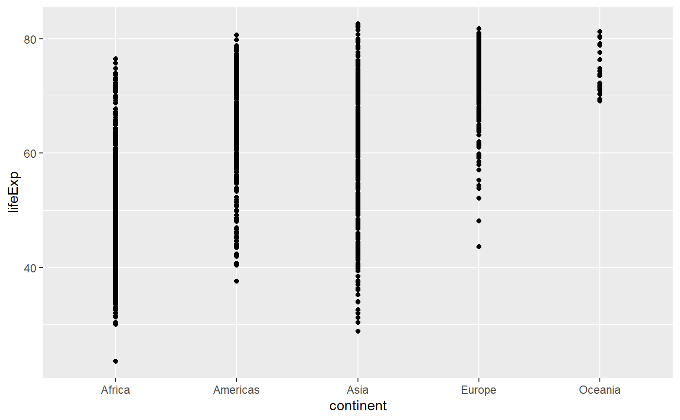
How can the same function make three different classes of plots?
One of the hidden arguments is geom which specifies the type of plot. The default is auto which leads to a guess of the plot type based on the data type(s) in the column(s) you specify.
Type ?qplot in the console to read the qplot documentation
Now let’s specify the type of plot explicitly
qplot(x = lifeExp, data = my_data, geom = 'histogram')
#> `stat_bin()` using `bins = 30`. Pick better value with `binwidth`.
# Note that we are now specifying boxplot instead of point plot
qplot(x = continent, y = lifeExp, data = my_data, geom = 'boxplot')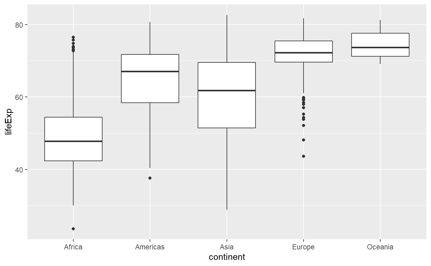
How to quickly make plots with qplot() that are easy to interpret
Now let’s change the number of bins in a histogram and make the plot prettier
# The hidden argument `bins` has a default valute of 30
qplot(x = lifeExp, data = my_data, geom = 'histogram')
#> `stat_bin()` using `bins = 30`. Pick better value with `binwidth`.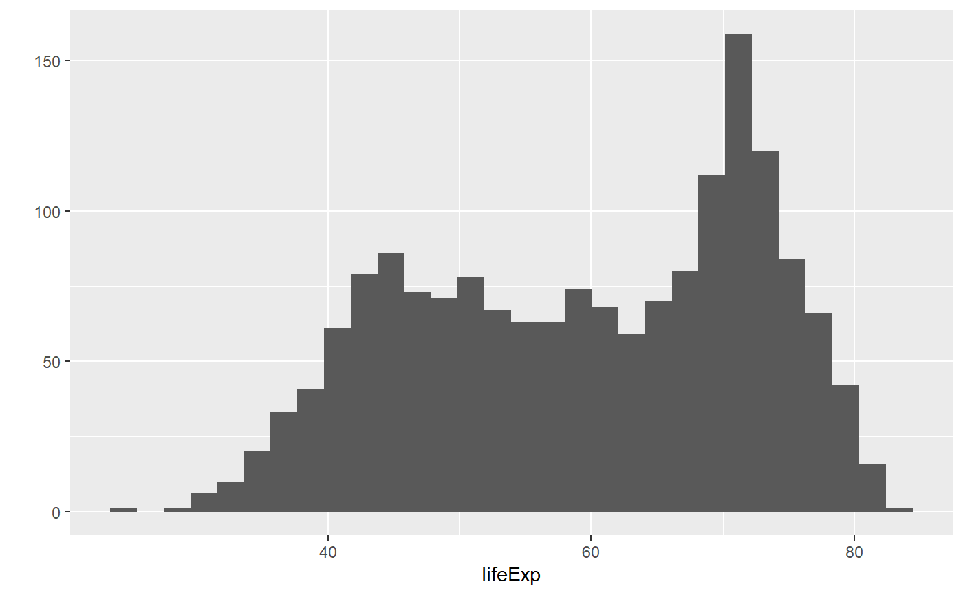
# This changes the number of bins to 10
qplot(x = lifeExp, bins = 10, data = my_data, geom = 'histogram')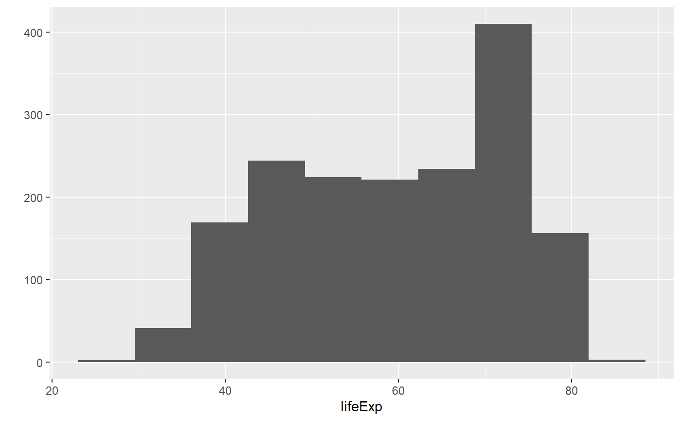
# Alternatively you can choose the width you want the bins to have
qplot(x = lifeExp, binwidth = 5, data = my_data, geom = 'histogram')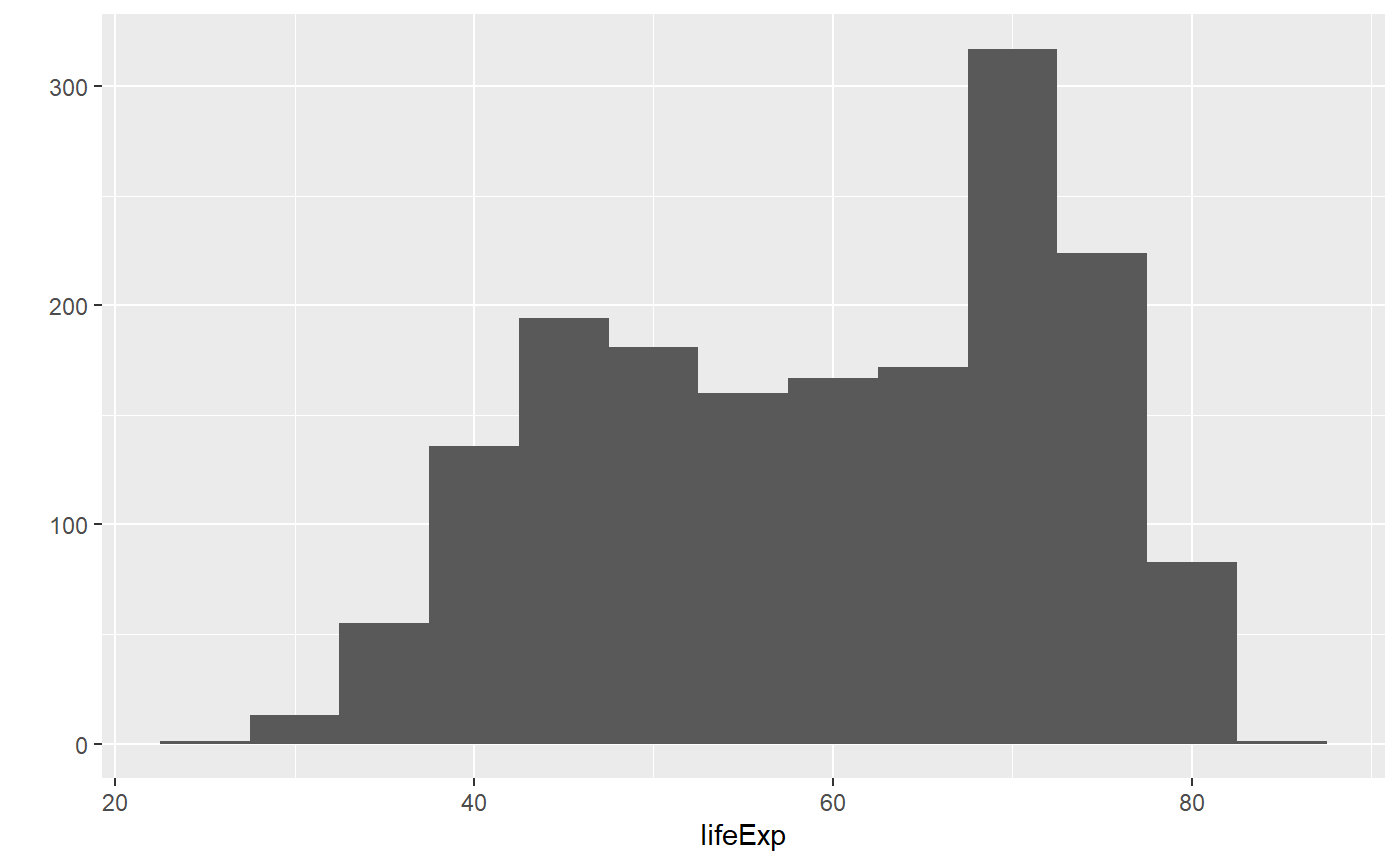
# Let's add a title
qplot(x = lifeExp, binwidth = 5, main = "Histogram of life expectancy", data = my_data, geom = 'histogram')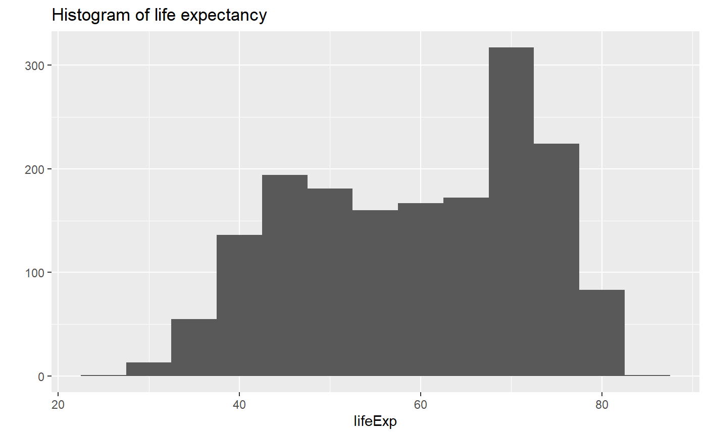
# Let's add an x axis label
qplot(x = lifeExp, binwidth = 5, main = "Histogram of life expectancy", xlab = "Life expectancy (years)", data = my_data, geom = 'histogram')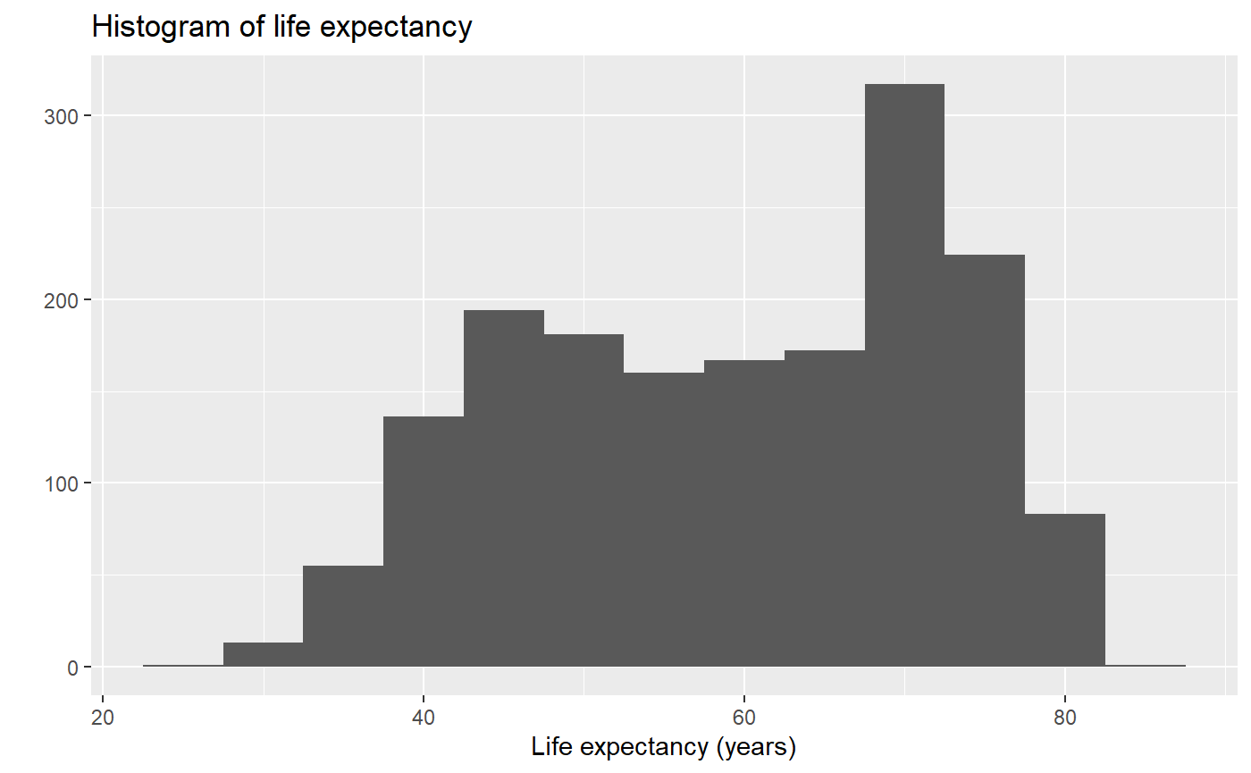
# Let's add a y axis label
qplot(x = lifeExp, binwidth = 5, main = "Histogram of life expectancy", xlab = "Life expectancy (years)", ylab = "Count", data = my_data, geom = 'histogram')
# This format is easier to read, but otherwise exactly the same.
# The convention is to break lines after commas.
qplot(x = lifeExp,
      binwidth = 5,
      main = "Histogram of life expectancy",
      xlab = "Life expectancy (years)",
      ylab = "Count",
      data = my_data,
      geom = 'histogram')
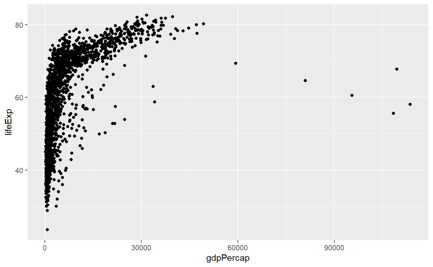
Log scale & trendline
Let’s apply a log scale and add a trendline to a scatter plot

# Here the x axis is log transformed
qplot(x = gdpPercap,
      y = lifeExp,
      log = 'x',
      data = my_data,
      geom = 'point')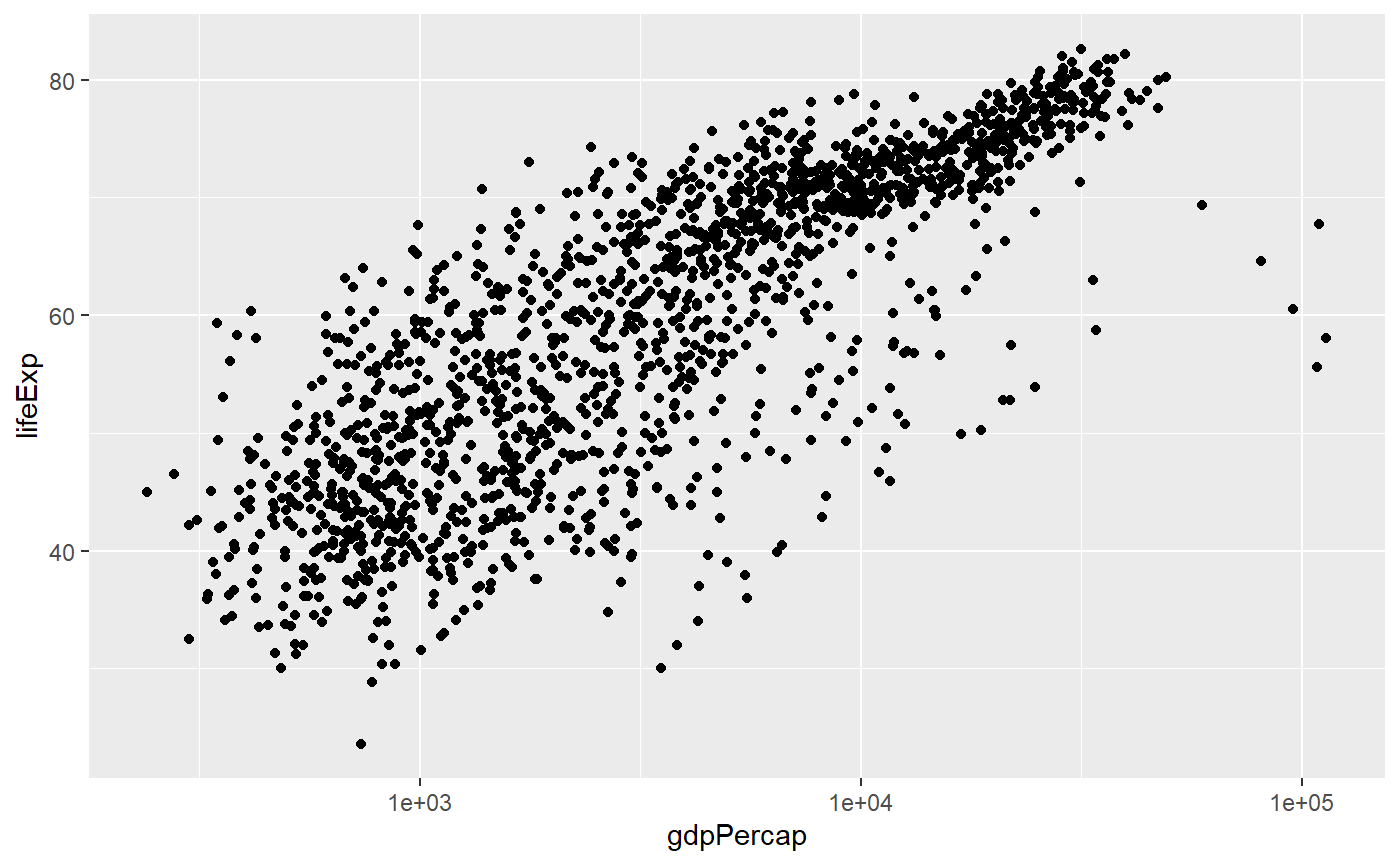
# Let's add a trendline to the data as well.
# The linear regression model (`lm`) will be added on top of our previous plot
qplot(x = gdpPercap,
      y = lifeExp,
      log = 'x',
      main = "Scatter plot of life expectancy versus GDP per capita",
      xlab = "Log-transformed GDP per capita ($)",
      ylab = "Life expectancy (years)",
      data = my_data,
      # The following line adds a `smooth` trendline
      # We want our regression to be a linear model, or `lm`
      method = 'lm',
      # the `c()` function allows us to pass multiple variables
      # to the `geom` argument
      geom = c('point','smooth'))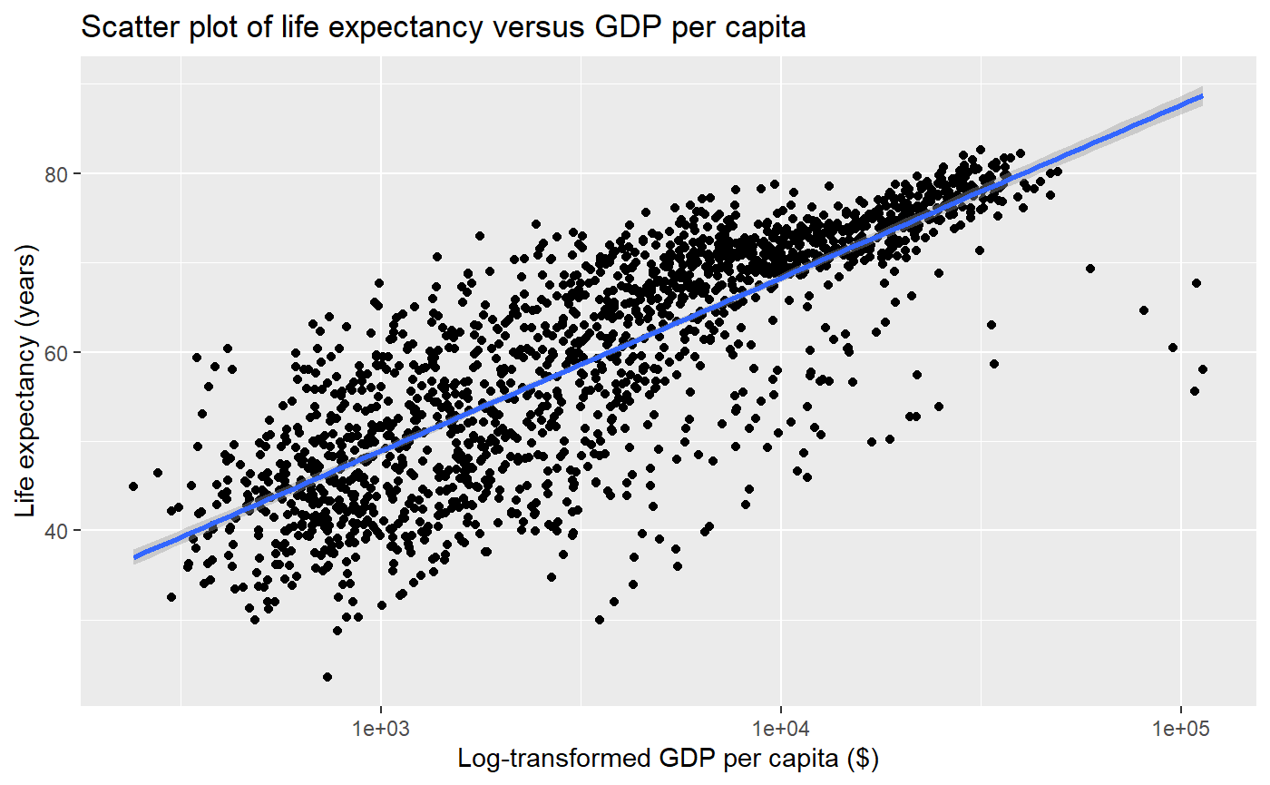
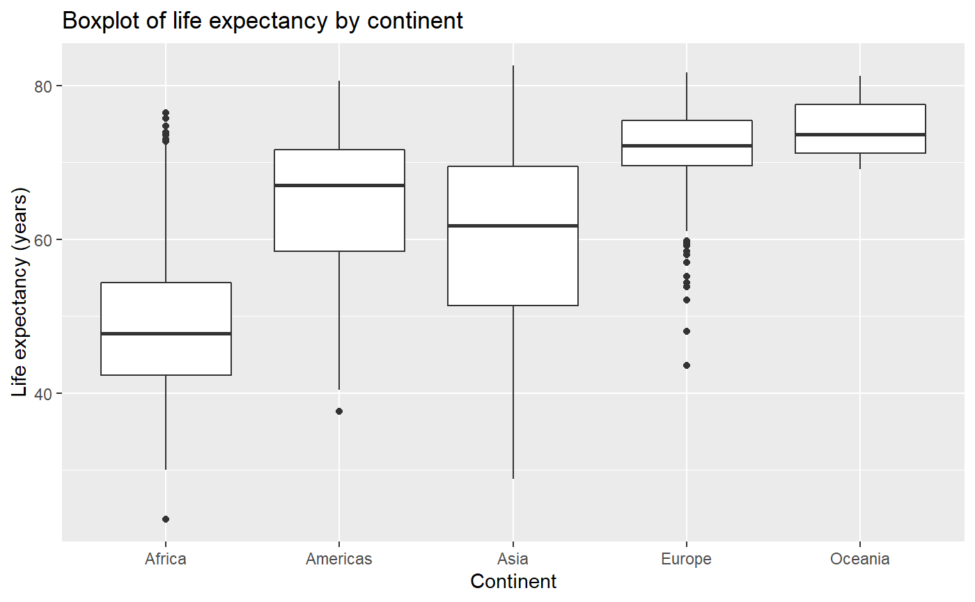
Building a boxplot using gapminder data
qplot(x = continent,
      y = lifeExp,
      main = "Boxplot of life expectancy by continent",
      xlab = "Continent",
      ylab = "Life expectancy (years)",
      data = my_data,
      geom = 'boxplot')